![]()
![]()
This is part a of a two part post. In this part we will look at the underlying theory behind simple linear regression and determining parameters for a line of best fit. In part b we will look at a worked example in q plus some statistics.
Linear regression is a supervised learning technique for predicting future numerical values based on historical data. The goal is to determine a optimal function which describes the trend in the data (when we have only one input and one output we call this finding the line of best fit). The sample data for linear regression is typically of the form:$$S=\{(\mathbf{x}_1,y_1),(\mathbf{x}_2,y_2),\dots,(\mathbf{x}_i,y_i),\dots,(\mathbf{x}_n,y_n)\}$$ where x i is a vector of inputs that describe the output y i:$$\mathbf{x}_i=\begin{pmatrix}x_{i0}\\x_{i1}\\\vdots\\x_{ii}\end{pmatrix}$$
The relationship between the independent variable x and dependent variable y for simple linear regression can be described with the following equation:$$h(\mathbf{x}_i)=y_i=\beta_0 x_{i0}+\beta_1 x_{i1}$$
For simple linear regression x i0 is always 1. This allows us to write the equation describing the relationship between x and y as:$$h(\mathbf{x}_i)=\beta\cdot\mathbf{x}_i=\beta_0+\beta_1x_{i1}$$
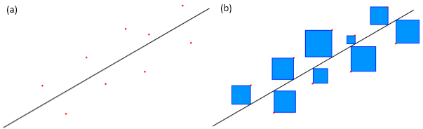
Once we have our function we need to find the optimal values of the parameters in the β vector which will give a function that produces the least error when applied to our sample data. This is done by using the least squares method. If we plot the current function approximation on the sample data (figure 1(a)) we can measure the residuals (the difference between the sample output and the output estimated by our function for the same input) and then square them (figure 1(b)). The motivation behind this is that the function which produces the smallest total area of these squares is the function with the best fit.
The equation for the sum of these squares is:$$J(\beta)=\sum^{n}_{i=1}(y_i-h(\mathbf{x}_i))^2$$ Where n is the total number of samples in the training set. We generalize this to multiple dimensions by writing the above equation in terms of matrices and vectors: $$J(\beta)=(\mathbf{y}-\mathbf{X}\beta)^T(\mathbf{y}-\mathbf{X\beta})$$Here y is a vector of all the target outputs and X is called the design matrix - a matrix whose rows are made of each input vector x i :$$\mathbf{y}=\begin{pmatrix}y_1\\y_2\\\vdots\\y_n\end{pmatrix};\mathbf{X}=\begin{pmatrix}\mathbf{x}_1^T\\\mathbf{x}_2^T\\\vdots\\\mathbf{x}_n^T\end{pmatrix}$$ Now all that is required is to minimize this function in terms of the parameter vector β. To find the minimum we differentiate with respect to β, set the result equal to 0 and solve for β: $$\mathbf{\beta}=(\mathbf{X}^T\mathbf{X})^{-1}\mathbf{X}^T\mathbf{y}$$ This equation is sometimes referred to as the Normal Equation. Onward to part b!